Explore application ready aggregated data - Grid of points
Application-ready-aggregated-data-grid-of-point.Rmd
library(climateChangeInAustralia)

library(stars)
#> Loading required package: abind
#> Loading required package: sf
#> Linking to GEOS 3.10.2, GDAL 3.4.1, PROJ 8.2.1; sf_use_s2() is TRUE
library(sf)
library(dplyr)
#>
#> Attaching package: 'dplyr'
#> The following objects are masked from 'package:stats':
#>
#>     filter, lag
#> The following objects are masked from 'package:base':
#>
#>     intersect, setdiff, setequal, union
library(tidyr)
library(forcats)
library(ggplot2)
library(units)
#> udunits database from /usr/share/xml/udunits/udunits2.xml
Application ready aggregated
See introduction to application ready data. The aggregated files contain Monthly, seasonal and annual data as time-series. They contain a single time value per range period (e.g. 2016-2045 has only 2031-01-01) per grid point (lat/lon), and then model values for monthly, seasonal and annual data (the remaining ‘columns’)
A small download
Here we will download Mean_Temperature for
2016-2045 for ACCESS1-0 and
rcp45, and then constrain to the the the Greater Sydney
Area bounding box using the included data object
greater_sydney_boundary
Get the boundary information.
# greater_sydney_boundary
load(system.file(package = 'climateChangeInAustralia', 'greater_sydney_boundary.rda'))

greater_sydney_boundary_bbox <-
  sf::st_bbox(greater_sydney_boundary)
Download the data. Note how the datetime_start have no effect …
ccia_dataset_urls <- ccia_dataset_urls()

dataset_url <-
  ccia_dataset_urls$
  application_ready_aggregated$
  Mean_Temperature$
  `2016-2045`$
  `tas_aus_ACCESS1-0_rcp45_r1i1p1_CSIRO-MnCh-wrt-1986-2005-Scl_v1_mon_seasavg_2016-2045_clim.nc`

dataset_query <-
  dataset_url |>
  ccia_create_dataset_request_url(access_type = ccia_access_types$NetcdfSubset) |>
  ccia_add_netcdf_subset_query(vars = 'all',
                               # Greater Sydney Area
                               bbox = greater_sydney_boundary_bbox,
                               # No effect (in this case)
                               datetime_start = '2016-01-01',
                               datetime_end = '2045-12-31',
                               datetime_step = 365)


dataset_download_filepath <-
  dataset_query |>
  ccia_perform_query(destfile = tempfile(fileext = 'tas_aus_ACCESS1-0_rcp45_seasavg_2016-2045.nc'))
#> file downloaded to: /tmp/Rtmp0oeGXr/file1c1c1bd7b54etas_aus_ACCESS1-0_rcp45_seasavg_2016-2045.nc

structure(
  file.size(dataset_download_filepath),
  class = 'object_size'
) |>
  format(units = 'MB')
#> [1] "0.2 Mb"
Import into R, wrangle and make a plot.
tas_ncdf <-
  dataset_download_filepath |>
  stars::read_stars()
#> tas_january, tas_february, tas_march, tas_april, tas_may, tas_june, tas_july, tas_august, tas_september, tas_october, tas_november, tas_december, tas_djf, tas_mam, tas_jja, tas_son, tas_ndjfma, tas_mjjaso, tas_annual,

tas_ncdf
#> stars object with 3 dimensions and 19 attributes
#> attribute(s):
#>                        Min.   1st Qu.   Median     Mean  3rd Qu.     Max. NA's
#> tas_january [C]   17.242945 21.650128 23.10048 22.59844 23.79595 25.15815  194
#> tas_february [C]  17.705004 21.852914 23.40874 22.85681 24.04764 25.31642  194
#> tas_march [C]     15.080417 19.063201 20.84573 20.29154 21.75056 22.67807  194
#> tas_april [C]     11.409605 15.251315 17.34300 16.86741 18.64882 20.03955  194
#> tas_may [C]        8.423323 12.119039 14.24687 13.82680 15.64040 17.40124  194
#> tas_june [C]       5.319645  9.247092 11.46520 11.00274 12.82167 14.76529  194
#> tas_july [C]       4.482938  8.355245 10.46848 10.15870 12.04739 14.12342  194
#> tas_august [C]     5.440468  9.606401 11.86455 11.35252 13.24449 14.83208  194
#> tas_september [C]  8.980540 13.067712 15.12566 14.59569 16.39969 17.46542  194
#> tas_october [C]   10.540699 15.060324 17.10557 16.45547 18.07766 18.92086  194
#> tas_november [C]  12.760968 17.539718 19.33781 18.67858 20.08645 21.26256  194
#> tas_december [C]  16.574490 21.051534 22.52772 22.00486 23.14145 24.53855  194
#> tas_djf [C]       17.155003 21.487839 22.99949 22.47038 23.65278 24.98917  194
#> tas_mam [C]       11.630178 15.449719 17.47408 16.98607 18.67635 19.98040  194
#> tas_jja [C]        5.117209  9.102658 11.28350 10.86230 12.72122 14.58578  194
#> tas_son [C]       10.754513 15.230988 17.22469 16.57557 18.17380 19.00014  194
#> tas_ndjfma [C]    15.113491 19.415837 21.12097 20.53441 21.91966 22.98969  194
#> tas_mjjaso [C]     7.205494 11.233259 13.41002 12.90277 14.72859 16.21136  194
#> tas_annual [C]    11.162054 15.366587 17.29219 16.72247 18.33499 19.27216  194
#> dimension(s):
#>      from to         offset delta  refsys x/y
#> x       1 35        149.925  0.05      NA [x]
#> y       1 28        -32.975 -0.05      NA [y]
#> time    1  1 2031-01-01 UTC    NA POSIXct
tas_ncdf_month <-
  # first 12 values are monthly estimates
  tas_ncdf[1:12] |>
  # merge attributes (temperatures) into a new dimension
  # and set it's values to month names
  merge() |>
  st_set_dimensions(4, values = month.name) |>
  # pop the time dimension
  split('time') |>
  # rename
  st_set_dimensions(names = c('x', 'y', 'time')) |>
  setNames('Temp')

# Match CRS to boundary for cropping (as it's missing also)
tas_ncdf_month <-
  tas_ncdf_month |>
  st_set_crs(value = st_crs(greater_sydney_boundary))
ggplot() +
  geom_stars(data = tas_ncdf_month[greater_sydney_boundary]) +
  facet_wrap(~time) +
  theme_void() +
  labs(title = 'Mean monthly temperature',
       subtitle = 'model: ACCESS1, scenario: rcp45')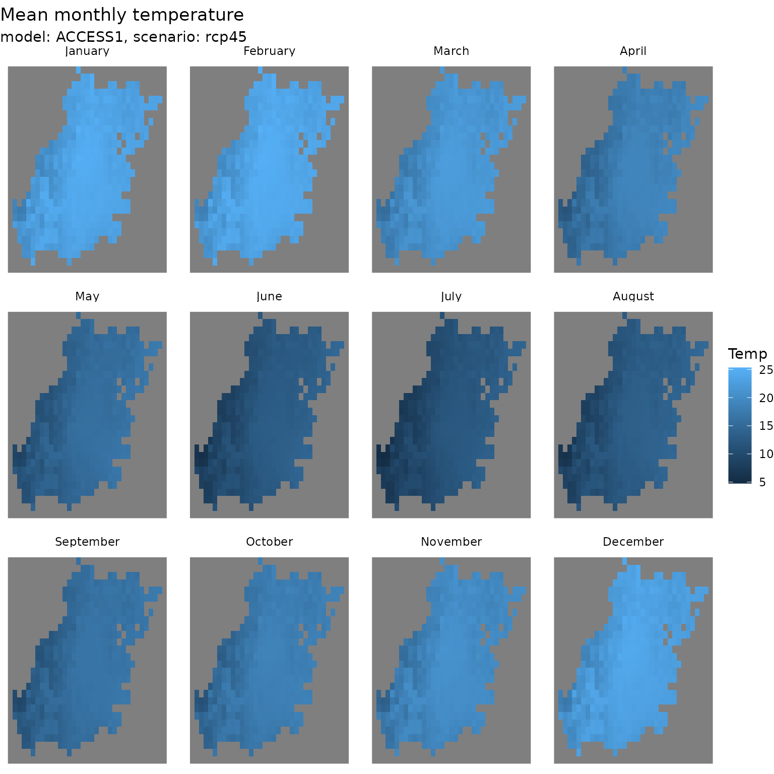
A time-series download
Needs a bit of R jujitsu ..
ccia_dataset_urls <- ccia_dataset_urls()

# Extract model 'ACCESS1-0_rcp85' through element names
series_urls <-
  lapply(ccia_dataset_urls$application_ready_aggregated$Mean_Temperature, function(urls){

    urls[grepl('ACCESS1-0_rcp85', names(urls))]

  })

# Expect 4 results
sapply(series_urls, names)
#>                                                                                      2075-2104
#> "tas_aus_ACCESS1-0_rcp85_r1i1p1_CSIRO-MnCh-wrt-1986-2005-Scl_v1_mon_seasavg_2075-2104_clim.nc"
#>                                                                                      2056-2085
#> "tas_aus_ACCESS1-0_rcp85_r1i1p1_CSIRO-MnCh-wrt-1986-2005-Scl_v1_mon_seasavg_2056-2085_clim.nc"
#>                                                                                      2036-2065
#> "tas_aus_ACCESS1-0_rcp85_r1i1p1_CSIRO-MnCh-wrt-1986-2005-Scl_v1_mon_seasavg_2036-2065_clim.nc"
#>                                                                                      2016-2045
#> "tas_aus_ACCESS1-0_rcp85_r1i1p1_CSIRO-MnCh-wrt-1986-2005-Scl_v1_mon_seasavg_2016-2045_clim.nc"

# Build requests
series_requests <-
  lapply(series_urls, function(url){

    url |>
      ccia_create_dataset_request_url(access_type = ccia_access_types$NetcdfSubset) |>
      ccia_add_netcdf_subset_query(vars = 'all',
                                   # Greater Sydney Area
                                   bbox = greater_sydney_boundary_bbox)
  })

# Download data
series_filepaths <-
  lapply(series_requests, function(req){

    filename <- sub('.*\\d/(.*\\.nc).*', '\\1', req$url)

    req |>
      ccia_perform_query(destfile = tempfile(pattern = 'ccia-', fileext = filename))

  })
#> file downloaded to: /tmp/Rtmp0oeGXr/ccia-1c1c3092dd30tas_aus_ACCESS1-0_rcp85_r1i1p1_CSIRO-MnCh-wrt-1986-2005-Scl_v1_mon_seasavg_2075-2104_clim.nc
#> file downloaded to: /tmp/Rtmp0oeGXr/ccia-1c1c38271f92tas_aus_ACCESS1-0_rcp85_r1i1p1_CSIRO-MnCh-wrt-1986-2005-Scl_v1_mon_seasavg_2056-2085_clim.nc
#> file downloaded to: /tmp/Rtmp0oeGXr/ccia-1c1c784cc002tas_aus_ACCESS1-0_rcp85_r1i1p1_CSIRO-MnCh-wrt-1986-2005-Scl_v1_mon_seasavg_2036-2065_clim.nc
#> file downloaded to: /tmp/Rtmp0oeGXr/ccia-1c1c4d3bb417tas_aus_ACCESS1-0_rcp85_r1i1p1_CSIRO-MnCh-wrt-1986-2005-Scl_v1_mon_seasavg_2016-2045_clim.nc
Import into R, wrangle and make some plota.
series_stars <-
  lapply(series_filepaths, stars::read_ncdf, var = 'tas_annual')
#> Will return stars object with 980 cells.
#> No projection information found in nc file.
#>  Coordinate variable units found to be degrees,
#>  assuming WGS84 Lat/Lon.
#> Will return stars object with 980 cells.
#> No projection information found in nc file.
#>  Coordinate variable units found to be degrees,
#>  assuming WGS84 Lat/Lon.
#> Will return stars object with 980 cells.
#> No projection information found in nc file.
#>  Coordinate variable units found to be degrees,
#>  assuming WGS84 Lat/Lon.
#> Will return stars object with 980 cells.
#> No projection information found in nc file.
#>  Coordinate variable units found to be degrees,
#>  assuming WGS84 Lat/Lon.

do.call(c, series_stars) |>
  plot(key.pos = 1,
       box_col = 0)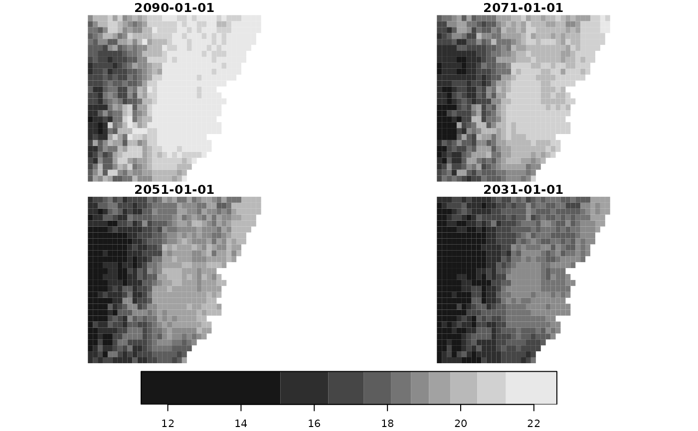
Monthly
month_var_names <- paste0('tas_', tolower(month.name))

series_stars <-
  lapply(series_filepaths, stars::read_ncdf, var = month_var_names)
#> Will return stars object with 980 cells.
#> No projection information found in nc file.
#>  Coordinate variable units found to be degrees,
#>  assuming WGS84 Lat/Lon.
#> Will return stars object with 980 cells.
#> No projection information found in nc file.
#>  Coordinate variable units found to be degrees,
#>  assuming WGS84 Lat/Lon.
#> Will return stars object with 980 cells.
#> No projection information found in nc file.
#>  Coordinate variable units found to be degrees,
#>  assuming WGS84 Lat/Lon.
#> Will return stars object with 980 cells.
#> No projection information found in nc file.
#>  Coordinate variable units found to be degrees,
#>  assuming WGS84 Lat/Lon.

wrangle_months <- function(x){

  year <-
    x |>
    st_get_dimension_values('time') |>
    format('%Y')

  x[month_var_names] |>
    merge() |>
    st_set_dimensions(4, values = paste(month.abb, year)) |>
    split('time') |>
    st_set_dimensions(names = c('x', 'y', 'time')) |>
    setNames('Temp')
}

series_stars_wrangled <-
  lapply(rev(series_stars), wrangle_months) |>
  do.call(what = c)

series_stars_wrangled <-
  series_stars_wrangled |>
  st_transform(crs = st_crs(greater_sydney_boundary))

series_stars_wrangled <-
  series_stars_wrangled[greater_sydney_boundary]
# downsampled for faster plotting
ggplot() +
  geom_stars(data = series_stars_wrangled, downsample = c(2,2,0)) +
  facet_wrap(~time, ncol = 4, dir = 'v') +
  theme_void()
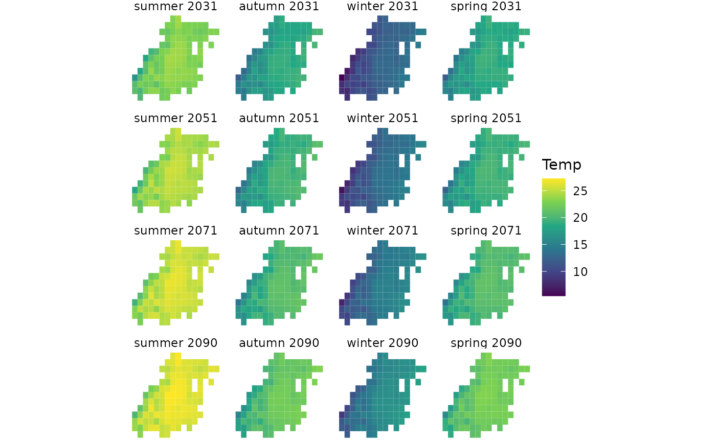
Seasonal
season_var_names <-
  c(summer = 'tas_djf',
    autumn = 'tas_mam',
    winter = 'tas_jja',
    spring = 'tas_son')

series_stars <-
  lapply(series_filepaths, stars::read_ncdf, var = season_var_names)
#> Will return stars object with 980 cells.
#> No projection information found in nc file.
#>  Coordinate variable units found to be degrees,
#>  assuming WGS84 Lat/Lon.
#> Will return stars object with 980 cells.
#> No projection information found in nc file.
#>  Coordinate variable units found to be degrees,
#>  assuming WGS84 Lat/Lon.
#> Will return stars object with 980 cells.
#> No projection information found in nc file.
#>  Coordinate variable units found to be degrees,
#>  assuming WGS84 Lat/Lon.
#> Will return stars object with 980 cells.
#> No projection information found in nc file.
#>  Coordinate variable units found to be degrees,
#>  assuming WGS84 Lat/Lon.

wrangle_seasons <- function(x){

  year <-
    x |>
    st_get_dimension_values('time') |>
    format('%Y')

  x[season_var_names] |>
    merge() |>
    st_set_dimensions(4, values = paste(names(season_var_names), year)) |>
    split('time') |>
    st_set_dimensions(names = c('x', 'y', 'time')) |>
    setNames('Temp')
}

series_stars_wrangled <-
  lapply(rev(series_stars), wrangle_seasons) |>
  do.call(what = c)

series_stars_wrangled <-
  series_stars_wrangled |>
  st_transform(crs = st_crs(greater_sydney_boundary))

series_stars_wrangled <-
  series_stars_wrangled[greater_sydney_boundary]

ggplot() +
  geom_stars(data = series_stars_wrangled, downsample = c(1,1,0)) +
  facet_wrap(~time, ncol = 4) +
  scale_fill_continuous(type = 'viridis') +
  theme_void()